A sideways look at economics
“It is tough to make predictions, especially about the future.” This pithy remark has been attributed variously to American baseball player Yogi Berra, Danish physicist Niels Bohr, and even Mark Twain. Regardless of origin, it can be readily applied to the science – or, as I shall argue, the art – of economic forecasting.
When attempting to predict future values of any economic time series it is worth giving at least some thought to its order of integration. Over some periods of time, some economic time series will be stationary: that is to say, they will have a constant, well-defined mean and variance. These series are said to be integrated of order zero, or I(0). Until the early 20th century, the note issue in most major economies was backed by gold or some other precious commodity. This meant that the price level was frequently stationary. Prices in general might rise one year, perhaps following a bad harvest, but in time the price level would return to its long-run average. That is because the supply of money, and therefore its price, was determined by the quantity of some precious commodity, which to a first approximation was fixed.
Other economic time series appear ‘difference stationary’. Although they are not stationary in their own right, their first difference, or more accurately their rate of change, might be. Since the abandonment of the Gold Standard, and its successor the Bretton Woods system of fixed exchange rates, all countries have come to rely on fiat money. Fiat money is intrinsically worthless, backed by nothing but trust among the public that the government of the day will not issue too much of it.[1] During the era of fiat money, and floating exchange rates, which began in the early 1970s, it is inflation, rather than the price level, that has appeared stationary, at least for some periods of time. The price level, in other words, has appeared difference stationary, or integrated of order one – I(1).
How might we begin to forecast a series that we believe is stationary, like inflation? A simple, but often effective approach is to assume that next period inflation will be a weighted average of what it is today, and what it is on average in the long run. One can enjoy a fair degree of success in forecasting a stationary economic time series by estimating an equation of the form:
χt = β0 + β1χt-1 + εt
Here χt is what’s known as an autoregressive process, because it depends only on lags of itself. In this case there is just one lag, so χt is autoregressive of order one, or AR(1). In the case where χt is inflation, β1 is the weight we put on today’s rate of inflation when forecasting inflation in the next period, and 1-β1 is the weight we put on its long-run average value.[2] εt is a random, unknowable shock, with a zero mean. It is one of the forecaster’s enemies. The larger is the variance of εt, the more we will struggle to forecast χt. Nevertheless, over the period from 2000 to 2019, an equation like the one above would have done an OK job when it comes to forecasting inflation in most major economies. It could, for example, have explained around 25% of the variation in UK inflation, rising to almost 60% with the addition of other potential explanatory variables such as an estimate of the output gap, and changes in commodities prices and the sterling exchange rate. In this respect, it easily beats the implicit forecasts of investors in the UK swaps market.[3] Using this approach, we would be exploiting the fact that, to the best of our knowledge, inflation has a constant, well-defined mean. If it’s above average in the current period, it ought to be lower, on average, in the next period.
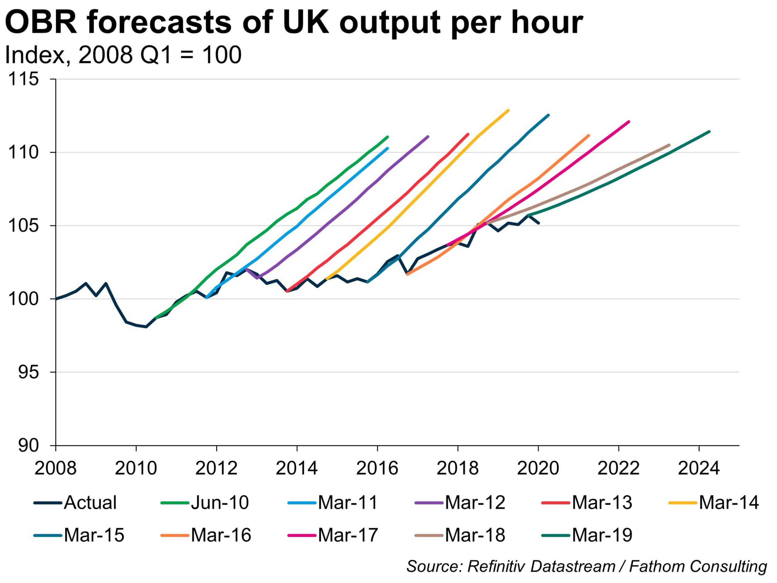
But sometimes using this simple approach will cause us to come unstuck. My first chart shows successive forecasts of the level of UK productivity made by the Office for Budgetary Responsibility (OBR) from its inception in 2010 through to the eve of the pandemic. Known (within Fathom at least) as a hedgehog chart, with successive forecasts representing the spines, and the actual outturn the back, it is a convenient graphical device for representing not just a bad set of forecasts, but the gradual process of learning. Around the time of the Global Financial Crisis (GFC), the trend rate of growth of labour productivity changed in more or less all major economies. It fell, in the case of the UK, from just over 2.0% per annum to less than 0.5% per annum. Over any sample period spanning the GFC, labour productivity was neither stationary, nor difference stationary. Standard forecasting techniques, that assume a stationary or difference stationary series, failed. In common with many other UK economy watchers, the OBR made systematic forecast errors year after year after year, finally throwing in the towel and recognising that the UK was not returning to its pre-GFC rates of productivity growth some ten years down the line.
The change in the average rate of labour productivity growth that took place around the GFC is an example of a structural break – the biggest enemy of any economic forecaster. Structural breaks can be hard to spot. Are we witnessing a series of unfortunate events – a run of bad economic shocks, in other words – or has the underlying economic process changed? That is the kind of question that we, as economists, must ask ourselves on a regular basis.
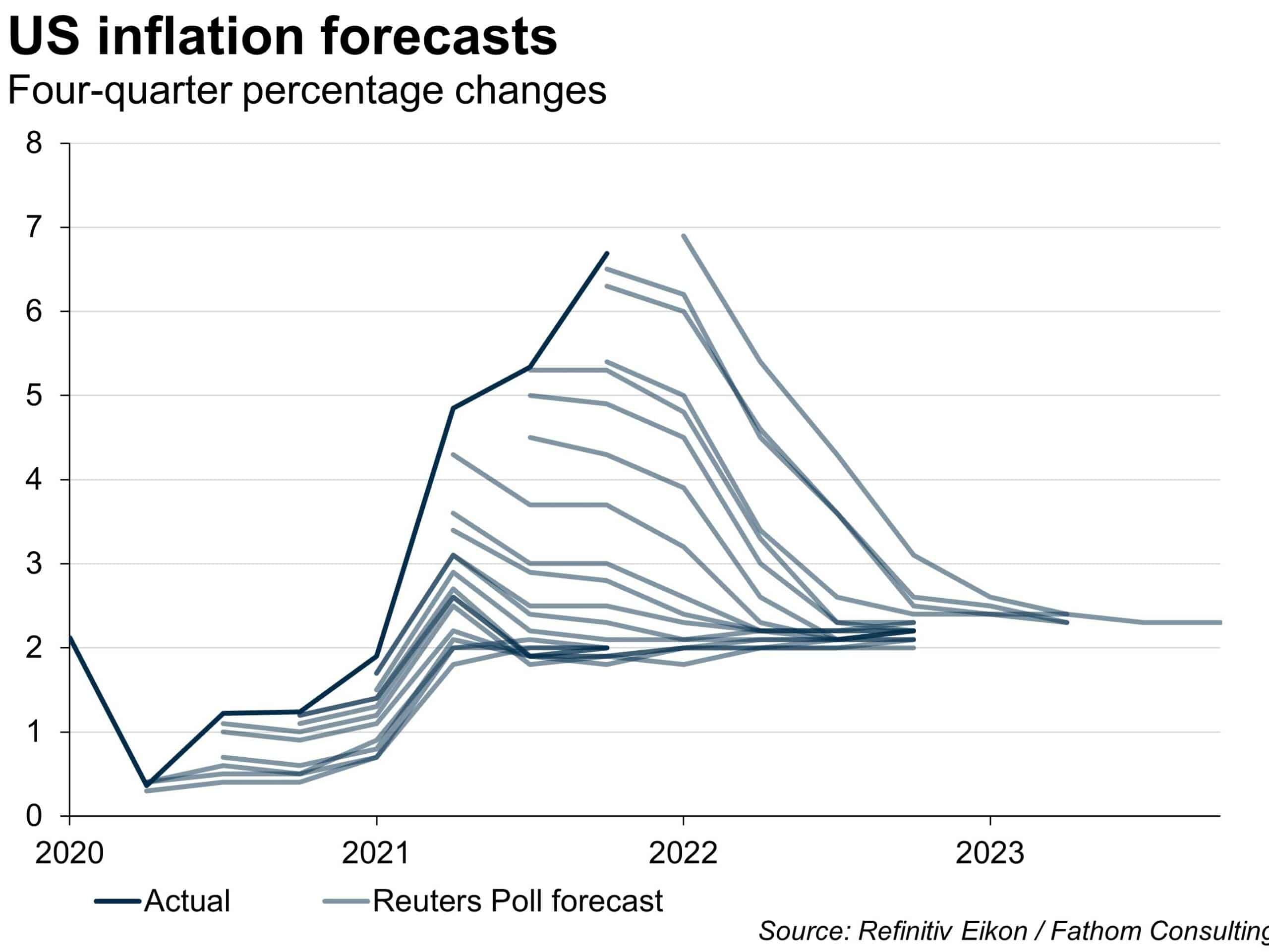
Let us return, finally, to the question of forecasting inflation. My second chart shows US CPI inflation outturns since the start of the pandemic, alongside successive forecasts of the same made by respondents to the Reuters Poll. Time and again, US inflation has surprised on the upside, and dramatically so through last year. Are we witnessing another structural break? Maybe. The difficulty with our simple equation above is that, in the case where χt is inflation, the coefficient β1, which measures the persistence of inflation, is not a deep structural parameter. It will depend on many factors that are prone to change, including human behaviours, and in particular the way in which wage- and price-setters form their beliefs about future inflation. For much of economic history, right up until the early 1970s, β1 was close to zero. It rose sharply during the early years of floating exchange rates, before falling back again as most major-economy central banks adopted credible inflation-targeting policies. In fact, the time series properties of inflation in most major economies from the early 1990s right up until at least the onset of the pandemic were very much as they had been under the Gold Standard. Following a shock that pushed inflation away from target, inflation would return very quickly back to the target. Are we still in that world? That is the key question for our upcoming Global Economic and Markets Outlook for 2022 Q2.
In truth, very few economic time series are stationary, or even difference stationary. For a period of time they may appear to be, until suddenly, they are not — which is why forecasting is as much an art as it is a science. It depends on judgement. To quote a former Bank of England governor: “Models don’t make forecasts. People do”.
[1] All Bank of England five pound notes carry the reassuring commitment: “I promise to pay the bearer on demand the sum of five pounds”. Ten, twenty and fifty pound notes all give similar assurances. What does this mean in practice? Not a great deal, though when I worked at the Bank it was a good excuse for tourists to come to the front door at Threadneedle Street and demand to exercise their rights as bearers of a Bank of England note. On doing so, they would be admitted, shown into the banking hall and allowed to exchange their five pound note for… another one.
[2] It can be shown that the long-run average value is given by β0/(1-β1). We know that β1 must be less than one as that is a necessary condition for stationarity.
[3] If I estimate an equation relating the current twelve-month inflation rate to the one-year inflation swap rate twelve months previously over the entire period for which I have data (from 2007 to the present day), the R-squared statistic is just 0.02. It turns out the one-year inflation swap tells you far more about inflation today than it does about inflation in one year’s time.