A sideways look at economics
I’m not a big football fan, though I do follow Brighton, to a degree. They are my local team, and back in the early 1980s, my dad used to take me to watch the odd game at the old Goldstone Ground — now a retail park. I also take a passing interest in statistics. It’s part of the job. And I have long had a suspicion that Brighton’s results are somewhat erratic. I think I can date this back to the 1982/83 season, when, having just been relegated from the old First Division, Brighton unexpectedly made it through to the final of the FA Cup. The big day dawned, and they drew 2-2 against Man Utd – a commendable result, but a game they should have won 3-2. The club fanzine, when such things existed, was named And Smith must score… after commentator Peter Jones’s excited pronouncement in the final moments of extra time. Smith didn’t score, and Brighton got hammered 4-0 in the replay. (There were no penalties in those days.)
These feelings of exasperation in response to Brighton’s seemingly almost random performances were reawakened towards the end of last season when, back in top-flight football, the Seagulls were vying for a place in Europe for the first time in the club’s history. With a 6-0 victory over Wolves at home in late April, things were looking good. They looked better still after a 1-0 victory, also at the Amex, to Man Utd (a team they had also beaten at Old Trafford – to see why this was particularly remarkable, read on). But then disaster struck, as Brighton were beaten 1-5 on home turf by Everton — a team fighting relegation. Was there no order to this? I resolved to investigate.
Having collected results from all 380 English Premier League (EPL) matches during the 2022/3 season, I estimated the following set of econometric equations, one for each club:[1]
![]()
Here x_gdif_yi is team x’s goal difference in their ith match against team y (i takes the value ‘1’ for the first match of the season and ‘2’ for the second). x_aggdif is team x’s aggregate goal difference across all 38 matches at the end of the season (unknown when the game takes place, of course), and y_aggdif is the same concept for team y. Brighton’s aggregate goal difference was 19 – so they scored 19 more goals than they conceded across all 38 games. (x_aggdif — y_aggdif) ought to be a measure of the relative ability of the two teams (we ignore the fact that this might change through the season). x_home_yi is a variable that takes the value ‘1’ if team x’s ith game against team y is played at home, and ‘-1’ if it is played away. Finally, ei is an error term, with zero mean and unknown variance. The larger is the variance of ei, the harder it is to predict the outcome of any match. In a nice, stable, predictable world, I would expect to find that β0 = 0, β1 = 1, and the variance of ei would be very small. With this set up, strong teams tend to beat weak teams, and they do so with a larger goal difference the greater is the difference in their abilities. Finally, β2 tells us about home advantage. If β2 is statistically significant and positive, it tells us that team x has a home advantage. They tend to perform better when playing at home, against any team, than they do when playing away. If β2 is statistically significant and negative, the reverse is true. If β2 is not statistically significant, one would conclude that, for team x, it makes no difference where the game is held.
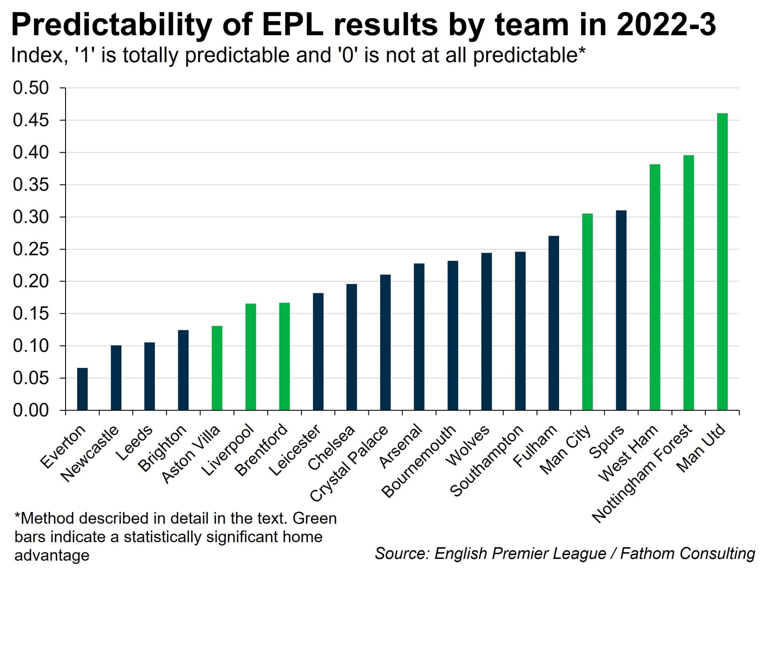
What did I find? Well, β0 was insignificantly different from zero for every team. β1 varied across teams, but was always positive, and often close to one. The results with regard to both the home advantage term ( β2) and the random element (ei) are summarised in the accompanying chart. Green bars are used to show teams that had a statistically significant home advantage. Fewer than half the teams fell into this category.[2]
What I was most interested in was the variance of ei. How big is the random element, and how does it vary across clubs? The height of each bar in my chart represents the R-squared statistic for each team, which in this case is an indicator of the predictability of that team’s results. For the case where R-squared = 1, the variance of ei is zero, and the outcome of each game can be predicted with complete certainty. For the case where R-squared = 0, the model tells us nothing at all about how that team will perform. You might as well toss a coin.
The results largely conform to my prior beliefs. While Everton’s results were, statistically, the hardest to call, Brighton was high up in the unpredictability rankings. There is genuine excitement to be had following Brighton – you really don’t know what’s going to happen from one game to the next. And the most boring team of all? No, not Arsenal, but Man Utd. Who’d have thought it?[3]
[1] For those who follow football even less closely than me, there are 20 teams in the EPL. Every team plays every other team twice. So every team plays 38 matches, and there are 380 matches in total.
[2] No teams had a statistically significant away advantage.
[3] Not only were Man Utd’s results the most predictable of the lot, they also had the largest home advantage, with the Red Devils likely to score almost two more goals (or concede two fewer goals) against any given team when the game was played at home rather than away. Some colleagues have speculated as to the potential cause of this substantial home advantage, but there is not space to go into that here.
More by this author